Google Analytics Data Mining With BigQuery And R
Big Query and Big Query Export for Google Analytics give us the power to visualize and explore virtually any trend in our GA data. It’s really quite powerful stuff. Because this tool is still very new, I want to get the conversation started on how advanced reporting can augment our digital analytics.
In this post I discuss data mining and the advanced reporting of Google Analytics data. I provide an R script for generating an E-commerce report with visualizations that are not possible within Google Analytics.
R script for Big Query E-commerce
My colleague Jonathan Weber has a nice article on Big Query and Google Analytics Data Export. Check this out for an overall refresher on Big Query, including billing information.
What are the Use Cases for Big Query in GA?
There are two big reasons to use Big Query to process and report on Google Analytics data:
- Sampling. Even for Premium customers, usage of advanced segments and non-standard secondary dimensions can lead to sampling. This can greatly affect the accuracy of quarterly, and even monthly, reporting.
- Data mining and advanced reporting. Google Analytics is, in our opinion at LunaMetrics, the best overall technology for digital analytics. But, like anything, it has its shortcomings. One of these is the customizability of reporting. GA’s ease of use and shallow learning curve also results in the need for additional tools for data mining and more-complex analysis.Cue Big Query. Our ability to generate complex metrics and mine trends is limited only by our knowledge of SQL. And the flexibility in visualizations by the limits of R, ShufflePoint, Tableau…a wide range of solutions.
Note: As a general cloud service, Big Query is not exclusive to GA Premium customers. However, Google Analytics Premium IS required in order to export complete GA data to Big Query. So, if you are not Premium, you can still upload data to Big Query and use it as a cloud solution for SQL-like data analysis. But you need Premium for working with GA data.
Questions about premium? See here for more information.
Overview of the Report
The R script should function out-of-the-box for any GA Premium customers with E-commerce data (and with the Big Query export enabled).
If you don’t have Google Analytics Premium, but are still interested in data mining and advanced reporting in for Google Analytics, you can still interface with R! Check out the R for Google Analytics library. By combining their starter template with the code for the graphs from my script, you should be able to achieve similar functionality. You will also need to conduct additional processing of this data in R, since you are unable to take advantage of the SQL-like querying of Big Query. Additionally, those with a high traffic volume in GA will likely experience sampling.
One last note. I owe a shout-out to Hadley Wickham for writing the Big Query R library.
Figure 1: Average pageviews with transaction versus without transaction
You could also get this information by using advanced segments in Google Analytics, but it’s nice to get it unsampled and to be able to generate box-and-whisker plots.
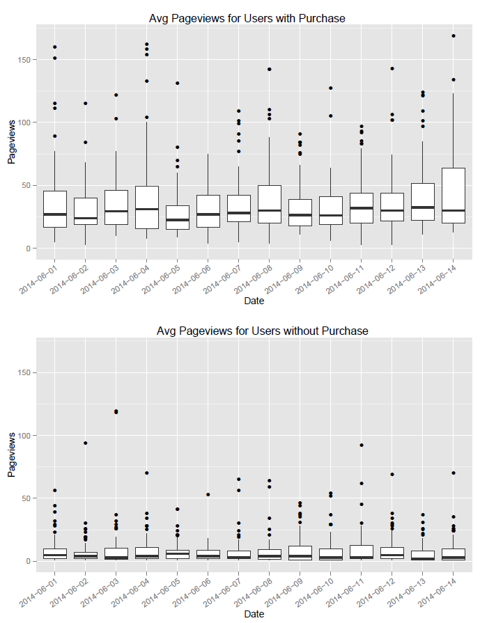
Figure 2: Average Revenue/Session by Medium
This is something you could calculate from Google Analytics, but that is not readily available as a metric. In this chart we graph two metrics simultaneously; average revenue is given by height, and the weight of each channel (sessions) is given by color.
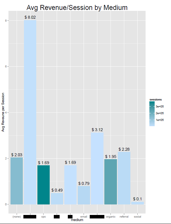
Figure 3: Top Campaigns by Revenue/Session
This chart is similar to the prior, except that we compare campaigns rather than medium. Again, the height shows the average revenue/session, and the color displays the weight of each campaign.
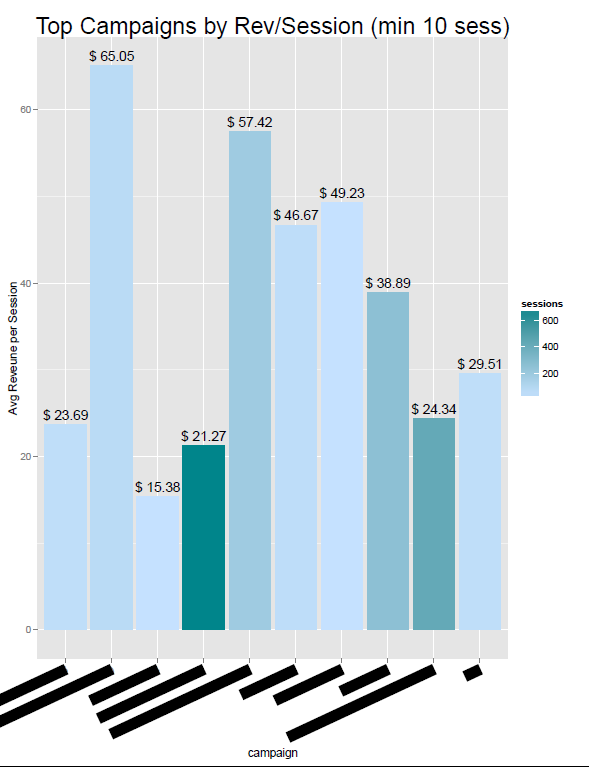
Figure 4: Product Category of Purchase by Medium (a)
Here, we group products purchased by their category. Then we break down the sales data for each category by medium.
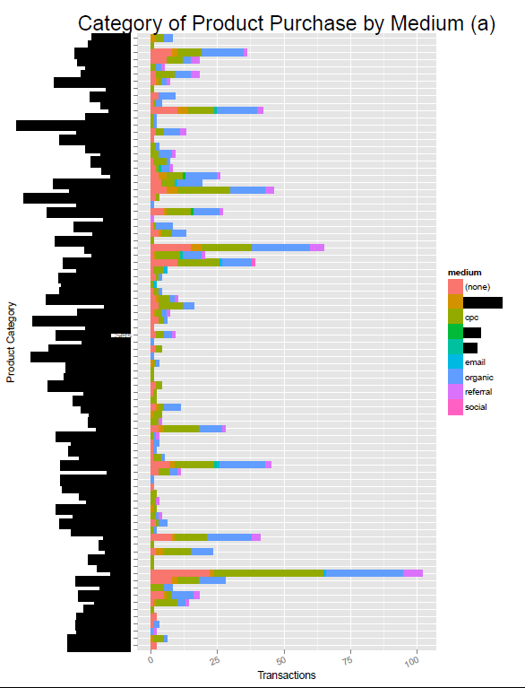
Figure 5: Product Category of Purchase by Medium (b)
This displays the same information as the prior chart, but visualized differently. The darkness of the tile indicates the number of products sold for a given product category and medium.
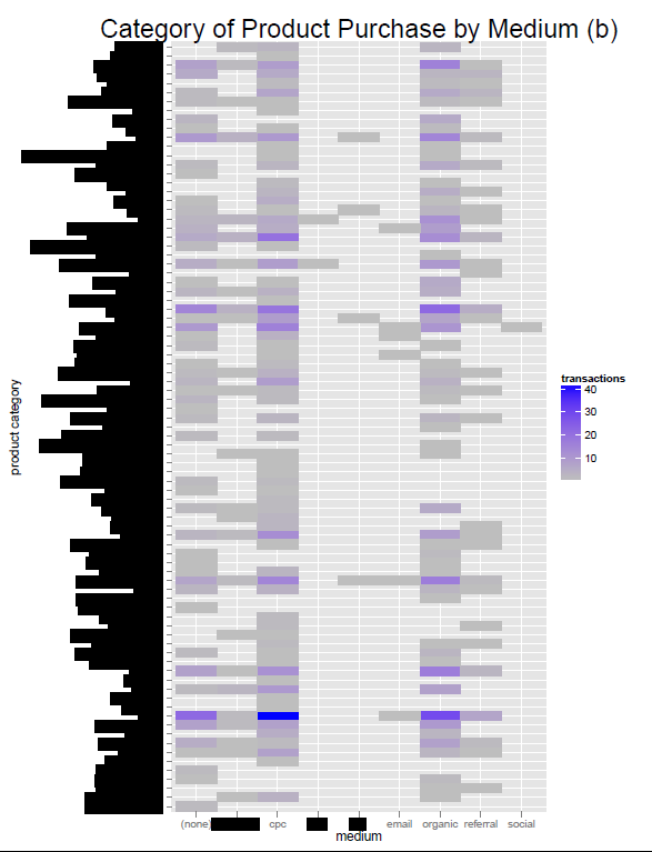
Figure 6: Likelihood of product to indicate and/or lead to additional transactions
This is my favorite chart. It is something we would never be able to calculate in Google Analytics. Here, we examine the products associated with a user’s initial transaction. We then calculate the percentage of users who made at least one additional transaction. And we segment this data by the initial product purchased. Thus, (pending a statistical test), we see that certain products may be indicators and/or causes of additional future purchases. Maybe they’re really great products and win the customer’s loyalty.
img id=”img6″ class=”alignnone size-full wp-image-12651″ src=”https://bounteous.com/wp-content/uploads/2014/06/page61.png” alt=”r-bigquery page 6″ width=”588″ height=”767″ />
R Script for Big Query E-commerce Report
install.packages('devtools')
install.packages('httpuv')

devtools::install_github("assertthat")
devtools::install_github("bigrquery")

library(bigrquery)
require(gridExtra)
require(ggplot2)


project <- "INSERT PROJECT ID HERE"
dataset <- "INSERT DATASET ID HERE"


#####################################
# Big Query queries
# note
# you also need to set your dataset id
# for TABLE_DATE_RANGE in each query
# below. replace "dataset" with the id
#####################################

sql1<- "SELECT date, totals.pageviews AS total_pageviews_per_user,
FROM (TABLE_DATE_RANGE([dataset.ga_sessions_], TIMESTAMP('2014-06-01'),
	TIMESTAMP('2014-06-14')))
WHERE totals.transactions >=1 AND totals.pageviews >=0
ORDER BY fullVisitorId LIMIT 1000"

data1 <- query_exec(project,dataset,sql1, billing = project)


sql2<- "SELECT date, totals.pageviews AS total_pageviews_per_user,
FROM (TABLE_DATE_RANGE([dataset.ga_sessions_], TIMESTAMP('2014-06-01'),
	TIMESTAMP('2014-06-14')))
WHERE totals.transactions IS NULL AND totals.pageviews >=0
ORDER BY fullVisitorId LIMIT 1000"

data2 <- query_exec(project,dataset,sql2, billing = project)


sql3 <- "SELECT trafficSource.medium AS medium, count(*) AS sessions,
sum(totals.transactionRevenue)/1000000 AS total_rev,
sum(totals.transactionRevenue)/(count(*)*1000000)
AS avg_rev_per_visit
FROM (TABLE_DATE_RANGE([dataset.ga_sessions_], TIMESTAMP('2014-06-01'),
TIMESTAMP('2014-06-07')))
GROUP BY medium
ORDER BY avg_rev_per_visit DESC LIMIT 10;"

data3 <- query_exec(project,dataset,sql3, billing = project)


sql4 <- "SELECT trafficSource.campaign AS campaign, count(*) AS sessions,
sum(totals.transactionRevenue)/1000000 AS total_rev,
sum(totals.transactionRevenue)/(count(*)*1000000)
AS avg_rev_per_visit
FROM (TABLE_DATE_RANGE([dataset.ga_sessions_], TIMESTAMP('2014-06-01'),
TIMESTAMP('2014-06-07')))
GROUP BY campaign HAVING sessions >= 10
ORDER BY avg_rev_per_visit DESC LIMIT 10;"

data4 <- query_exec(project,dataset,sql4, billing = project)


sql5 <- "SELECT trafficSource.medium AS medium,
hits.item.productCategory AS category, count(*) as value
FROM (TABLE_DATE_RANGE([dataset.ga_sessions_],
	TIMESTAMP('2014-06-01'),
TIMESTAMP('2014-06-02'))) WHERE hits.item.productCategory IS NOT NULL
GROUP BY medium, category
ORDER BY value DESC;"

data5 <- query_exec(project,dataset,sql5, billing = project)


sql7 <- "
SELECT prod_name, count(*) as transactions
FROM
(
SELECT fullVisitorId, min(date) AS date, visitId,
hits.item.productName as prod_name
FROM (
SELECT fullVisitorId, date, visitId, totals.transactions,
hits.item.productName FROM
(TABLE_DATE_RANGE([dataset.ga_sessions_], TIMESTAMP('2014-06-01'),
TIMESTAMP('2014-06-14')))
)
WHERE fullVisitorId IN
(
SELECT fullVisitorId
FROM (TABLE_DATE_RANGE([dataset.ga_sessions_], TIMESTAMP('2014-06-01'),
TIMESTAMP('2014-06-14')))
GROUP BY fullVisitorId
HAVING SUM(totals.transactions) > 1
)
AND hits.item.productName IS NOT NULL
GROUP BY fullVisitorId, visitId, prod_name ORDER BY fullVisitorId DESC
)
GROUP BY prod_name ORDER BY transactions DESC;"
data7 <- query_exec(project,dataset,sql7, billing = project)


sql8 <- " SELECT hits.item.productName AS prod_name,
count(*) AS transactions
FROM (TABLE_DATE_RANGE([dataset.ga_sessions_],
	TIMESTAMP('2014-06-01'),
                       TIMESTAMP('2014-06-14')))
WHERE hits.item.productName IS NOT NULL
GROUP BY prod_name ORDER BY transactions DESC;"

data8 <- query_exec(project,dataset,sql8, billing = project)


#################################
#processing
#################################

data9 <- merge(data7,data8,by.x="prod_name",by.y="prod_name")
data9$perc <- data9$transactions.x/data9$transactions.y
data9 <- data9[with(data9, order(-transactions.y, perc)), ]
data9 <- data9[1:10,]


##################################
# BEGIN PLOTTING
##################################

pdf("my first bigquery-r report.pdf",width=8.5,height=11)

y_max <- max(max(data1$total_pageviews_per_user),
max(data2$total_pageviews_per_user))/2

#plot 1
p1<- ggplot(data1, aes(paste(substr(date,1,4),"-",substr(date,5,6),"-",
	substr(date,7,8),sep=""),total_pageviews_per_user)) + geom_boxplot()
p1 <- p1 + labs(title="Avg Pageviews for Users with Purchase",
	x = "Date", y = "Pageviews")
p1 <- p1 + ylim(c(0,y_max))
p1 <- p1 + theme(axis.text.x = element_text(angle = 35, hjust = 1))

#plot 2
p2<- ggplot(data2, aes(paste(substr(date,1,4),"-",substr(date,5,6),"-",
	substr(date,7,8),sep=""),total_pageviews_per_user)) + geom_boxplot()
p2 <- p2 + labs(title="Avg Pageviews for Users without Purchase",
	x = "Date", y = "Pageviews")
p2 <- p2 + ylim(c(0,y_max))
p2 <- p2 + theme(axis.text.x = element_text(angle = 35, hjust = 1))

grid.arrange(p1,p2,nrow=2)


#plot 3
par(mfrow=c(1,1))
p3<- ggplot(data3, aes(x = medium,y=avg_rev_per_visit,
	fill=sessions,label=sessions))+
geom_bar(stat="identity")+scale_fill_gradient(low = colors()[600],
	high = colors()[639])
p3 <- p3 + geom_text(data=data3,aes(x=medium,
	label=paste("$",round(avg_rev_per_visit,2)),
	vjust=-0.5))
p3 <- p3+ labs(title="Avg Revenue/Session by Medium", x = "medium",
 y = "Avg Reveune per Session")
p3 + theme(plot.title = element_text(size = rel(2)))


#plot 4
par(mfrow=c(1,1))
p4<- ggplot(data4, aes(x = campaign,y=avg_rev_per_visit,fill=sessions,
	label=sessions))+geom_bar(stat="identity")+
scale_fill_gradient(low = colors()[600], high = colors()[639])
p4 <- p4 + geom_text(data=data4,aes(x=campaign,label=paste("$",
	round(avg_rev_per_visit,2)),vjust=-0.5))
p4 <- p4 + labs(title="Top Campaigns by Rev/Session (min 10 sess)",
 x = "campaign", y = "Avg Reveune per Session")
p4 <- p4 + theme(plot.title = element_text(size = rel(2)))
p4 + theme(axis.text.x = element_text(angle = 25, hjust = 1))


#plot 5
par(mfrow=c(1,1))
p5 <- qplot(category,data=data5, weight=value, geom="histogram",
	fill = medium, horizontal=TRUE)+coord_flip()
p5 <- p5 + labs(title="Category of Product Purchase by Medium (a)",
 x = "Product Category", y = "Transactions")
p5 <- p5+ theme(plot.title = element_text(size = rel(2)))
p5 + theme(axis.text.x = element_text(angle = 25, hjust = 1))


#plot 6
par(mfrow=c(1,1))
p6 <- ggplot(data5, aes(medium,category)) + geom_tile(aes(fill=value))+
scale_fill_gradient(name="transactions",low = "grey",high = "blue")
p6 <- p6 + labs(title="Category of Product Purchase by Medium (b)",
	x = "medium", y = "product category")
p6 + theme(plot.title = element_text(size = rel(2)))


#plot 7
par(mfrow=c(1,1))
p7<- ggplot(data9, aes(x = prod_name,y=perc,fill=transactions.y,
	label=perc))+
geom_bar(stat="identity")+scale_fill_gradient(name="transactions",
	low = colors()[600], high = colors()[639])
p7 <- p7 + geom_text(data=data9,aes(x=prod_name,
	label=paste(round(perc*100,1),"%"),vjust=-0.5))
p7 <- p7 + labs(title="Percentage of Transactions resulting in Future rn
	Additional Transactions by same User", x = "Product Name",
	y = "Percentage of Transactions")
#p7 <- p7 + theme(plot.title = element_text(size = rel(2)))
p7 + theme(axis.text.x = element_text(angle = 45, hjust = 1))


dev.off()


