Getting Started With ShufflePoint

Overview
ShufflePoint is a paid application that uses Excel’s built-in “Web Query” function to pull data from Google Analytics into Excel. It is an extremely powerful tool and allows you to take advantage of Excel’s data manipulation abilities. This gives you the freedom to develop compelling visuals that will help you quickly assess the performance of a website. When I was developing my first ShufflePoint report, I found that thinking about and planning data organization took the most time. My hope is that this article will help you graph your Google Analytics data in Excel with as little trial and error as possible.
Setting up a ShufflePoint Query
Before you can pull data from your Google Analytics account you will need to log into ShufflePoint and generate a key for your Google Analytics Property and a Profile (View) ID for the view you want to pull data from. Once you have those two things you can start setting up your Excel Spreadsheet.
To get started, mimic the image below when setting your first spreadsheet. First, add your key and Profile ID and designate a spot where you’ll enter a ‘Start Date’ and ‘End Date’ for your data pull. Under the start and end dates, add a place for the ‘Timeframe’ function which will format the dates to be compatible with ShufflePoint. In the empty cells below, you can enter your first query.

Here is an explanation of what all those things are:
- The Account Key- This key is specific to a single account in Google Analytics and in conjunction with the profile ID is what allows you to call data from the API. All you need to know is you need one. Once you put it in your workbook you’ll never touch it again.
- Profile ID- This is a number ShufflePoint generates based on the view you would like to pull data from.
- Timeframe- This is where to specify the period of time for the report. The most important thing to remember is that formatting matters. The timeframe format must look like this: yyyy-mm-dd:yyyy-mm-dd where the first date is the start date and the second date is the end date. That formatting is not very user-friendly- if you need to change the date on a regular basis it can become an inconvenience. Instead, we can use the formula below to format normal dates into the correct shuffle point range.
Here is what it looks like: =CONCATENATE(TEXT(F5,”yyyy-mm-dd”),”:”,TEXT(G5,”yyyy-mm-dd”)).
Example: I know my start data needs to be 01-01-2014 and my end data to be 07-31-2014. Instead of entering it into that wonky format you can just use the concatenate function to reference one cell that is the start date and another that is the end date. Seems like I’m making things more complicated than they need to be, right? When we look at its application, you’ll see why this is useful.
- Actual application: I open my Excel sheet on September 2nd with the intent to run an August report. Knowing that I’ll always open this document to run the previous month’s report, I create an equation that finds the end date of last month. That equation is: =EOMONTH(TODAY(),-1). To find the start date, I then reference that end date and count back however many months of data I want. *Be careful of sampling here. ShufflePoint doesn’t tell you if your data is sampled so it is a good idea to double-check that your preferred timeframe doesn’t show skewed data. I like to use 18 months when I can. This allows me to see year-over-year comparisons and an additional six months which is great if your website is affected by seasonality. The start date equation for 18 months of data looks like this: =EDATE(G5+1,-18) where G5 is not an airplane but a reference for to the end date.
After you have the Key, Profile, and Timeframe set up you are ready start building queries! Queries have four main parts: metrics, dimensions, a timeframe (FROM) and a filter.
Queries are outlined as such:
- SELECT
- METRICS
- DIMENSIONS
- FROM default
- WHERE FILTER
METRICS & DIMENSIONS: A great resource for metrics and dimensions is in Google’s API documentation. You can search for common metrics and dimensions found in the GA interface. Note: not all metrics and dimensions are in this list, the API can be restrictive in this way. Double-check before you go plugging-in metrics into your spreadsheet. You must have at least one dimension listed and you are able to use up to 10 metrics.
FROM: ‘From’ can be used to dictate a comparison timeframe. ShufflePoint has options for last week, last month, last year, etc. I prefer to keep this as ‘default’ and do comparisons by running a second query for a different timeframe. This makes for cleaner data sets which makes the data easier to work with in Excel.
WHERE FILTER: Here you can use include/exclude equations to slice and dice the data you want. Filters can be any metric or dimension that Google uses in their API- it is not restricted by the metrics and dimensions in your query. Just like filters in Google Analytics, you can use include, exclude and REGEX (regular expressions) when filtering data. Here are example equations:
- Include: ga:region==”Pennsylvania”
- Exclude: ga:region!=”Pennsylvania”
- Regex Include: ga:landingPagePath!~”/blog/.*” excludes blog traffic data
- Include Regex: ga:landingPagePath=~”/blog/.*” includes only blog traffic
Query Organization
Knowing how many rows of data will be pulled is crucial to how you will organize your queries. The basic rule of thumb is: if you don’t know how many rows will be pulled, run the query in its own tab. When ShufflePoint pulls data, it writes it into the rows of Excel. So if you’re unsure how many rows of data it’s going to pull, you have the potential for overwriting another query. For instance, I have a ShufflePoint workbook that pulls multiple sets of 18-month data which I pull in a single tab. That same workbook has multiple landing page queries where each are on their own tab.
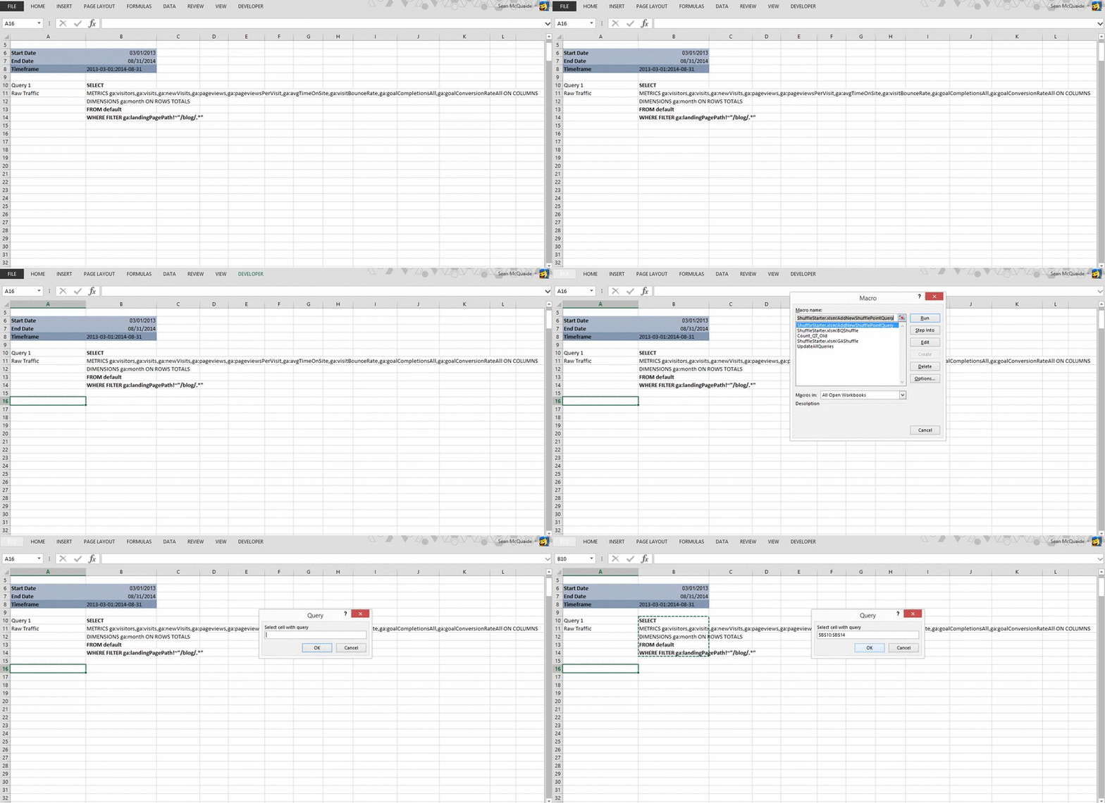
To make the process simpler and more efficient, we have developed a macro to help you with setting up your queries. Download the workbook and have it open when you are setting up your queries. First select the cell where you want to data to begin. Then run the ShuffleStarter macro. This ShuffleStarter macro is in beta, so leave a comment if you have a problem with it.

Now you can easily and quickly report on Google Analytics data in Excel! Once you can pull basic data, you can experiment with different filters, segments, and combinations of metrics. You may even gain unique insights and trends that may have been missed in the Google Analytics interface.


