Marketing Channel Attribution With Markov Models In R

Data empowers us to better understand our users and their behaviors, while methods provide us with the means for analysis. These methods, ranging anywhere from simplistic (i.e. frequency) to complex (i.e. clustering), allow us to choose what we want to understand from the data.

A popular way to understand our users and their behaviors in Google Analytics is through multichannel attribution in the Multi-Channel Funnels Reports using simple heuristics: First Click, Last Click, and Linear Attribution. Although these methods respectively provide insight into the frequency of the first marketing touchpoint, the frequency of the last marketing touchpoint, or a sequence of equally important marketing touchpoints, a data consumer may want a different snapshot. For instance, someone who wants to understand the level of importance and/or the value of each touchpoint in relation to conversions must use a different method: Markov modeling.

Just a few, quick reasons to use this method…

1. If you don’t have Google Analytics 360, then you don’t have access to the Data-Driven Attribution Model.
2. Even if you do have GA360, the Data-Driven Attribution algorithm is a bit of a blackbox.
3. You can use any sequenced data – you are not limited to only using marketing channels.

Let’s dive in!

The Make of Markov

A Markov model determines the probability that a user will transition from Sequence A to Sequence B based on the steps that each user takes through a site. The contents of these sequences are determined by the Markov order, which ranges from 0 to 4. Use the following as an example:

• Order 0: Doesn’t know where the user came from or what step the user is on, only the probability of going to any page.
• Order 1: Looks back zero steps. You are currently at Step A (Sequence A). The probability of going anywhere is based on being at that step.
• Order 2: Looks back one step. You came from Step A (Sequence A) and are currently at Step B (Sequence B). The probability of going anywhere is based on where you were and where you are.
• Order 3: Looks back two steps. You came from Step A > B (Sequence A) and are currently at Step C (Sequence B). The probability of going anywhere is based on where you were and where you are.
• Order 4: Looks back three steps. You came from Step A > B > C (Sequence A) and are currently at Step D (Sequence B). The probability of going anywhere is based on where you were and where you are.

Markov models account for user paths that extend past the order number by acting like a sliding window. Let’s say that User X’s steps were as follows: A > B > C > D > E > F > G. This model would show User X going from Sequence A (A > B > C > D) to Sequence B (B > C > D > E) to Sequence C (C > D > E > F), and so on until User X either exited or converted.

Choosing the best Markov order can be difficult. Without getting into a lot of detail, one way is to plot the training accuracy of the model versus the training standard deviation. The goal is to find where these two lines intersect, or where the model gains variability and loses accuracy equally.

Although it may appear daunting, having a basic understanding of the math behind the model can be helpful as well.

Luckily, this can be simplified into 3 main parts:

1. The Transition Probability (w_ij) = The Probability of the Previous State (Sequence A, X_t-1) Given the Current State (Sequence B, X_t)
2. The Transition Probability (w_ij) is No Less Than 0 and No Greater Than 1
3. The Sum of the Transition Probabilities Equals 1 (Everyone Must Go Somewhere)

The Make of ChannelAttribution

ChannelAttribution, an R library, builds the Markov models that allow us to calculate the number of conversions and/or conversion value that can be attributed to each marketing channel. In other words, ChannelAttribution uses Markov models to determine each channel’s contribution to conversion and/or value.

This model focuses on solving the following issues:

1. Objectivity – No gut feelings here! Only facts.
2. Predictive Accuracy – Predicts conversion events.
3. Robustness – Valid and reliable results.
4. Interpretability – Transparent and relatively easy to interpret.
5. Versatility – Not dataset dependent. Able to adapt to new data.
6. Algorithmic Efficiency – Provides timely results.

It’s also important to keep in mind the following limitations of attribution:

1. Endogenic – Attribution is relative to underlying conditions.
2. Not Strict Causal Interpretation – Markov models do not explain 100% of the variance between marketing channel contributions. For instance, certain marketing channels may be inherently more effective in a given setting.

This library estimates the channel attribution by calculating the Removal Effect (s_i). Essentially, the Removal Effect is the probability of converting when a step is completely removed; all sequences that had to go through that step are now sent directly to the exit node. This calculation is done by running a large number of simulations on the Markov model with the removed step. By default, it runs 1 million simulations. This occurs for each step present in the data.

ChannelAttributionApp – A GUI

If you aren’t too familiar with R, but you’d still like to take advantage of what ChannelAttribution has to offer, there’s still hope! Or, if you would rather see the code, click here.

Use it on the shinyapp server by following this link: https://adavide1982.shinyapps.io/ChannelAttribution.

The link should bring you to the following:

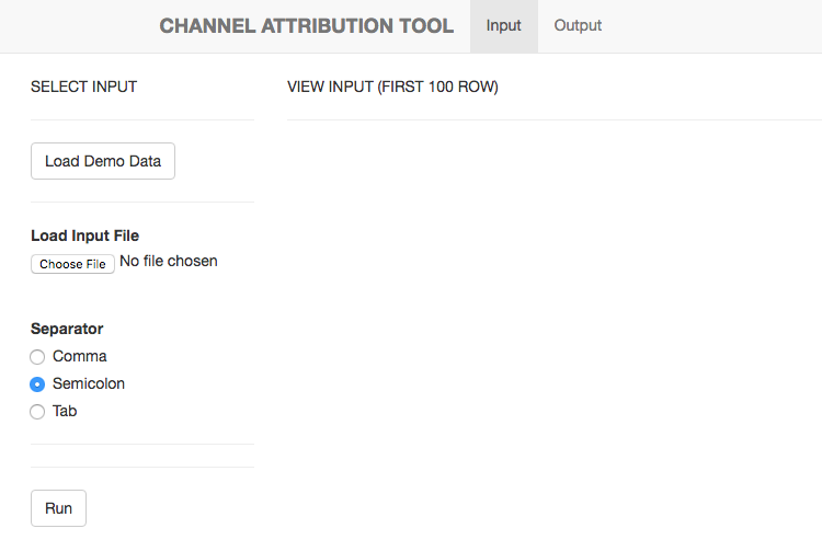
As shown in the image, click the “Load Demo Data” button (when you’re ready, you can load your own data by clicking the “Choose File” option under “Load Input File”).

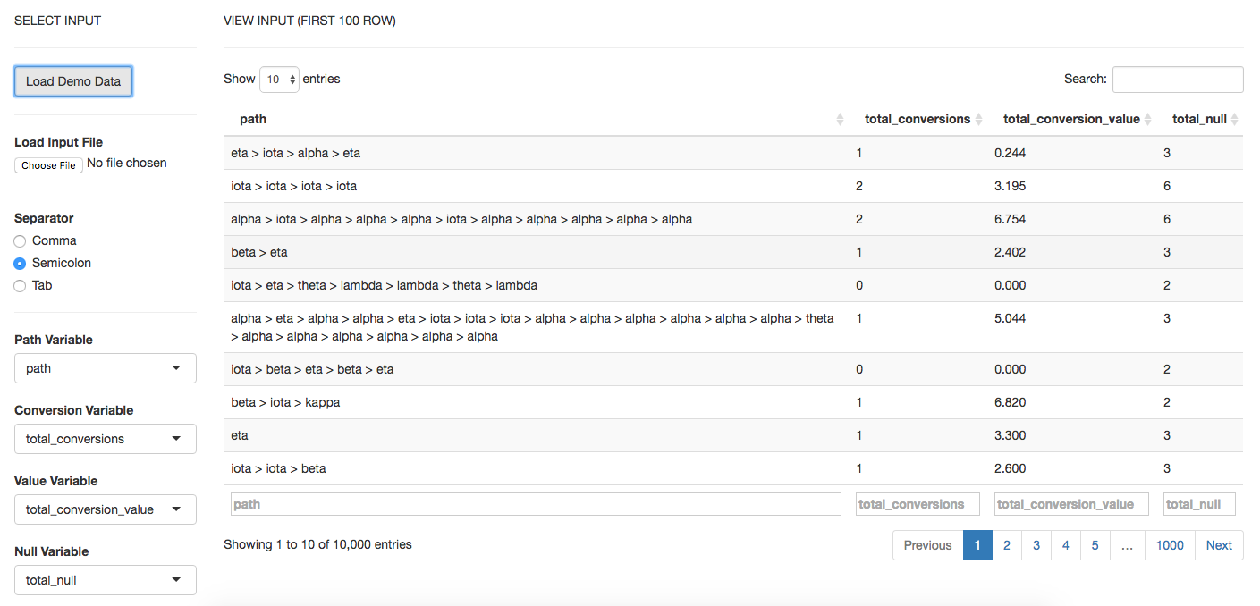
If you’re using the demo data, the options are preselected for your convenience. Otherwise, you will need to choose the delimiter that separates the values in your data. Then you fill in the column names for your variables:

• Path Variable – The steps a user takes across sessions to comprise the sequences.
• Conversion Variable – How many times a user converted.
• Value Variable – The monetary value of each marketing channel.
• Null Variable – How many times a user exited.

Then you hit “Run”! After it’s done executing (check the top right corner for progress), click on the “Output” tab. Analyze your results. In a lot of cases, you can see where this model is helpful … in some models, they give too little attribution to the channel versus they give too much attribution to the channel. Click here to jump to analysis section, complete with the bar charts and table from the output.

ChannelAttribution – R Code

If you’re more familiar with R, you might like this option better as you can customize your model and graphs. To get started, follow these steps:

Install and load ChannelAttribution, reshape, and ggplot2. Then load the demo data (or your own):

# Install these libraries (only do this once)
install.packages("ChannelAttribution")
install.packages("reshape")
install.packages("ggplot2")

# Load these libraries (every time you start RStudio)
library(ChannelAttribution)
library(reshape)
library(ggplot2)

# This loads the demo data. You can load your own data by importing a dataset or reading in a file
data(PathData)

Next, remind yourself of the variables used in calculating the models:

• Path Variable – The steps a user takes across sessions to comprise the sequences.
• Conversion Variable – How many times a user converted.
• Value Variable – The monetary value of each marketing channel.
• Null Variable – How many times a user exited.

Build the simple heuristic models (First Click / first_touch, Last Click / last_touch, and Linear Attribution / linear_touch):

H <- heuristic_models(Data, 'path', 'total_conversions', var_value='total_conversion_value')

# NOTE: If you want to use your own data, simply replace "Data" with the name of the object that's storing 
# your data. For instance, if I had a dataset stored in a variable called "myOwnData", the code would look 
# something like this:

H <- heuristic_models(myOwnData, 'path', 'total_conversions', var_value='total_conversion_value')

Build the Markov model (markov_model):

M <- markov_model(Data, 'path', 'total_conversions', var_value='total_conversion_value', order = 1) 
# You can specify the Markov order by adding the "order" argument. By default, it will run as Order 1.

# NOTE: The same steps apply from building the heuristics models in order to pass in your own data for building the markov_model.

Perform some quick data munging for total conversions:

# Merges the two data frames on the "channel_name" column.
R <- merge(H, M, by='channel_name') 

# Selects only relevant columns
R1 <- R[, (colnames(R)%in%c('channel_name', 'first_touch_conversions', 'last_touch_conversions', 'linear_touch_conversions', 'total_conversion'))]

# Renames the columns
colnames(R1) <- c('channel_name', 'first_touch', 'last_touch', 'linear_touch', 'markov_model') 

# Transforms the dataset into a data frame that ggplot2 can use to graph the outcomes
R1 <- melt(R1, id='channel_name')

And now the fun part... Plotting the total conversions:

# Plot the total conversions
ggplot(R1, aes(channel_name, value, fill = variable)) +
  geom_bar(stat='identity', position='dodge') +
  ggtitle('TOTAL CONVERSIONS') + 
  theme(axis.title.x = element_text(vjust = -2)) +
  theme(axis.title.y = element_text(vjust = +2)) +
  theme(title = element_text(size = 16)) +
  theme(plot.title=element_text(size = 20)) +
  ylab("")

# NOTE: The "+" allows you to split the code over multiple lines without running each line individually.

Thankfully, the process of creating the Total Value bar chart is very similar to creating the Total Conversions bar chart:

R2 <- R[, (colnames(R)%in%c('channel_name', 'first_touch_value', 'last_touch_value', 'linear_touch_value', 'total_conversion_value'))]

colnames(R2) <- c('channel_name', 'first_touch', 'last_touch', 'linear_touch', 'markov_model')

R2 <- melt(R2, id='channel_name')

ggplot(R2, aes(channel_name, value, fill = variable)) +
  geom_bar(stat='identity', position='dodge') +
  ggtitle('TOTAL VALUE') + 
  theme(axis.title.x = element_text(vjust = -2)) +
  theme(axis.title.y = element_text(vjust = +2)) +
  theme(title = element_text(size = 16)) +
  theme(plot.title=element_text(size = 20)) +
  ylab("")

The Long-Awaited Bar Charts, Table, and Brief Analysis

Total Conversions

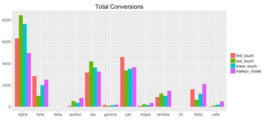
The "Total Conversions" bar chart shows you how many conversions were attributed to each channel (i.e. alpha, beta, etc.) for each method (i.e. first_touch, last_touch, etc.). Analyzing the graph, specifically the purple bar(markov_model) in comparison to the other methods, you can gain insights, such as the following:

• "alpha" was not actually as important in assisting conversions than the simple heuristics found.
• "epsilon", "lambda", "theta", and "zeta" were more important in assisting conversions than the simple heuristics found.

Total Conversion Value

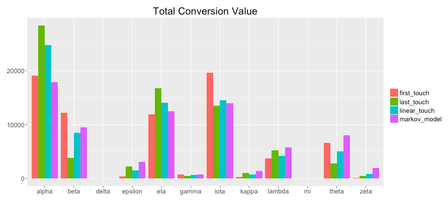
The "Total Conversion Value" bar chart shows you monetary value that can be attributed to each channel from a conversion.

For instance, you can see the following:

• "alpha" was not actually not as valuable in assisting conversions than the simple heuristics found.
• "epsilon", "lambda", "theta", and "zeta" were more valuable in assisting conversions than the simple heuristics found.

Table Form - Available via ChannelAttributionApp (GUI)

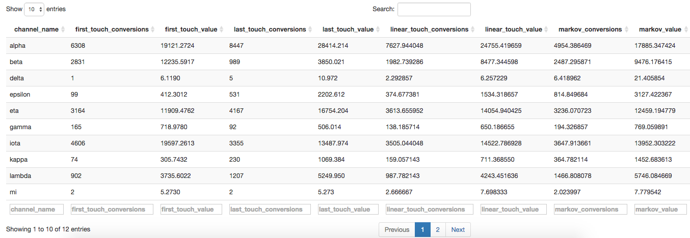
Furthermore, the GUI puts all this data into a table that you can download and open in Excel if you want to create your own charts.

Open in Excel

Although you can download the table and open it in Excel, it comes in semi-colon separated values. To convert this into usable data, you can follow these steps:

Select Column A. Then on the Data tab, click "Text to Columns". It will bring up the following prompt:

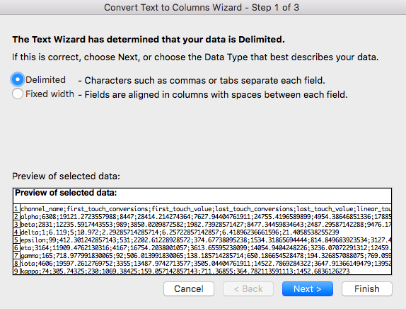
Select "Delimited" and click "Next".

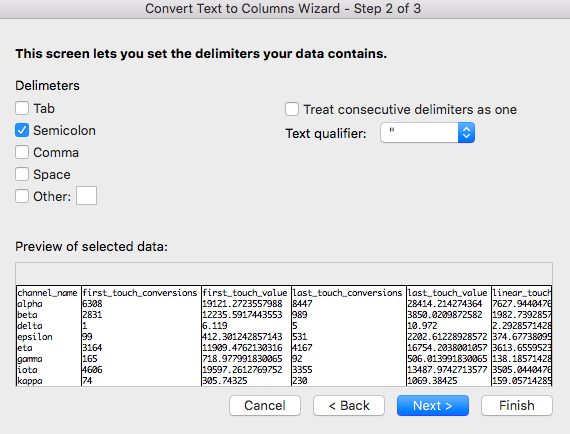
Make your bar charts again from there.

Choose the "Delimiter". In this case, it is the semicolon. Click "Finish". From here, you can create custom charts to your liking.

Opportunities Abound!

Now that you can get a better understanding of your Google Analytics marketing channel data, there is room to explore additional features of ChannelAttribution, reshape, and ggplot2. Bear in mind that although this library is mainly used for channel attribution issues, you can use it for almost any sequenced data. So get creative, and maximize your data's potential!